TRANSKRYPCJA VIDEO
Zach Star
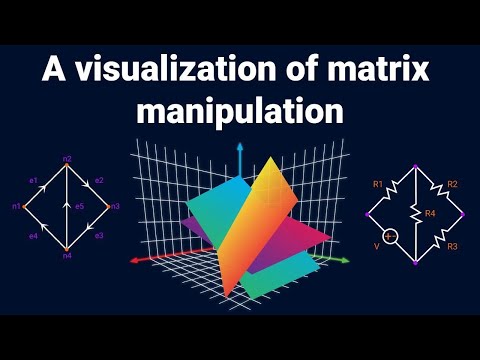
Dear linear algebra students, This is what matrices (and matrix manipulation) really look like
Opis wygenerowany przez Skrybot
In this informative video, you will learn about the fascinating world of linear algebra and how matrices can be used to solve systems of linear equations. You will discover two different ways to visualize solutions, either by finding the intersection of planes or by adding column vectors together to find scale factors. The video also introduces the concept of null space, which represents all possible solutions where all equations equal zero. You will learn how Gaussian elimination can be used to simplify the system of equations and determine dependent variables. The video also discusses the dot product of vectors and how it can be used to determine if two vectors are perpendicular.
Furthermore, you will explore the concepts of null space, row space, and column space in linear algebra and their applications in solving systems of equations and understanding networks in graph theory. The video discusses the concept of elimination, row and column spaces, and their applications in circuits and graph theory. You will learn that every connected graph reduces to a tree and how certain rows or edges that create loops eventually reduce to all zeros. The column space is what all the columns can combine to or any possible output vector b from a linear combination of these vectors. Kirchhoff's voltage law emerges from analyzing the column space of the matrix.
If you're interested in learning more about linear algebra, Brilliant.org offers courses covering adjacency matrices, graph theory, and the Google PageRank algorithm, as well as differential equation series covering underdamped systems, matrix exponentials, and more advanced topics. Don't miss out on this fascinating subject and dive into the world of linear algebra today!
Transkrypcja wygenerowana przez Skrybot
This video is sponsored by Brilliant. Every matrix paints some kind of picture, while matrix manipulation or arithmetic tells a story. And that's not just the one of how boring this can be in school. At least for me, the beginning of matrices was one of my least favorite parts of math. So I wanted this to at least show you what this all looks like with cool 3D software, as well as an application I never learned in school. So here we go. When you're given a matrix, it can often be useful to think of it as a set of vectors.
I'll be working mostly with 3x3 matrices, and you can think of these both as a set of 3 column vectors, or 3 row vectors. We'll look into each. Where the column vectors come in immediately is when we use this matrix to represent a system of equations. Here I'm sure most of you know this gives you three linear equations. For example, the first is 1x plus 2y plus 4z equals some b1. And the rest of the matrix is all the other coefficients. But another way to visualize this same thing is to write it as a sum or linear combination of the column vectors, where x, y, and z are now just scale factors.
Here the first equation would be 1 times x plus 2 times y plus 4z equals b1. The exact same thing. So given some system to solve, you can visually think of this two ways. For the first option, you say, if I were to graph each of these, or in this case three planes, where do they all intersect? Because that intersection is our solution x, y, z, and in this case it'd be 1, 1, 1. Now I'm going to switch to Geogebra real quick because it's better for vectors. But the second option says to instead take the columns of our matrix and consider them as vectors.
Then find which scale factors are needed such that those vectors add tip to tail to get some other vector b1, b2, b3. So instead of an intersection, we're looking for scale factors. And in this case all of them would be 1. Just add the vectors together as they are. Thus 1, 1, 1 is our solution, just like we saw before. So we have two totally different visualizations for the exact same question. I like using the intersection one when I have to solve for x, y, and z. But when I'm asked what are the possible outputs here for b, then I like thinking of vectors.
Now I'm going to change the matrix just a bit and also make the b vector all zeros. This then changes the other equations, and now let's go back to the 3D plot. Here we have the first and third equation, and unless they're parallel, two different planes will always intersect in a line. Now if the remaining plane happens to intersect that same line as well, which it does, then we have an entire set of solutions x, y, and z such that all these equations are zero. The name we give to those solutions is the null space. It's just the intersection of all your equations when they equal zero.
Often that solution is just 0, 0, 0, but sometimes there's more. Here the null space is one dimensional, just a line in 3D space. Now on your homework you wouldn't graph three planes, most likely. You'd do something like Gaussian elimination, where you take two equations, multiply one or both by a constant, and cancel out one of the variables. But instead of just multiplying by negative 2 immediately, I'm going to sweep the constant from 0 to negative 2, and watch what happens to the resultant function, which currently is just that second graph in pink.
So look, you can see when you add any two of these linear equations, regardless of the scale factor in front, their intersection, or the null space in this case, is preserved. The new plane just rotates about that intersection. So we may have a totally different plane here, but we haven't lost the solutions, so we can just replace either equation 1 or 2 and still go through with the analysis. But now the arithmetic is a little easier because one of the coefficients is 0. If you do the same thing with equations 1 and 3, then one plane actually becomes another. This happens because if we replace equation 3, these last two planes are the exact same now.
That means if we were to continue the elimination, we get a row of all 0s. And for square matrices at least, a single row of 0s means we have a single free variable. This tells us we have infinitely many solutions to the system, and we say z can be anything, it's free. But x and y depend on that value, so we don't just have any solution. Those dependent variables correspond to something called pivots. And since there's only one free variable, then our null space will be one-dimensional.
And by the way, if we did have three planes that only intersect at a single point, then the elimination eventually leads to a plane of one variable, like in this case z equals 1. And from there we would back solve to get y and x. But anyways, now I want to complete the picture by putting back the original equations and graph. Now what if I told you that the dot product of the vector 1,2,4 and some random vector x,y,z is 0? Well, that means these two vectors are perpendicular. But look, the actual dot product, or 1x plus 2y plus 4z equals 0, is our first equation. And x,y,z represents the null space, that line of solutions.
So our equation says the first row vector of our matrix, 1,2,4, is perpendicular to the null space. And the second equation says the second row vector is also perpendicular to that same line, and same with the third. These are all just dot products being equal to 0. And the set of all vectors perpendicular to the null space line is this plane here. And the set of all vectors perpendicular to the null space line is this plane here. And this is what we call the row space. This is always perpendicular to the null space. It contains the three row vectors, all three are in that plane.
And it also contains every linear combination of those row vectors. So we have a one-dimensional null space and a two-dimensional row space, which add to three. And that matches this dimension of the matrix. Just note that this will always be true. But don't forget these equations, which represent planes, and now we know also dot products with the null space, can also be thought of as a combination of the column vectors. Since this is the exact same question, we already know there are x,y,z solutions to this that sum to the zero vector. It's just all the values that made up that null space line from before.
So there are infinitely many scale factors that make this work. And when a set of vectors can combine to the zero vector, given scale factors that aren't all zero, then those vectors are linearly dependent. Or you can also say one of these vectors is just a linear combination of the other two. Same thing. When you have a square matrix with linearly dependent vectors, it means those vectors don't span the entire space they're in. They're confined to like a line, or in this case, a plane. All the column vectors are found here, and also all of their linear combinations, all possible tip-to-tail summations.
The name we give to that plane that the vectors span is the column space. See, often you could put any three vector here and find a solution, which would mean the vectors are linearly independent. But in the dependent case, we can't have any solution. The output vector has to lie within this plane, the column space, in order for a solution to exist. The column space and the row space, which I'll throw in here as well, usually look very different, but they're always the same dimension. Both are 2D in this case. For non-square matrices, the row and column space are way different. Here, the column space is just the xy plane.
These four vectors can only combine to some other x,y vector. But the row space is the plane spanned by these two vectors in four-dimensional space. However, both those spaces are planes that are themselves two-dimensional, so that aspect does match. But graphically, these are very different. Now, with regards to elimination, the obvious reason as to why this is important is because it's used to solve systems of equations. When there are many of those equations, which can come up in circuits or other physical systems, then we might not solve things by hand, but we do have to tell computers how to get a solution.
However, there's even more of a picture and story beyond just solving these equations, and that has to do with graph theory and networks. Let's say we have some directed graph with four nodes and five connecting edges, and I'll actually label all these edges E1 through 5 and the nodes N1 through 4. Now, you can think of this like a circuit, where the edges are either resistors or a battery or whatever where current flows, and the nodes would all have some specific voltage. In fact, I'll change the labels to voltages to stay consistent with this.
Then the arrows would sort of represent current, although we can't know the direction yet, until at least here we know if the voltage is positive or negative. Now, we can represent this network with something called an incidence matrix that will have four columns for the four nodes and five rows for the five edges. To fill this in, just consider the first edge. On the graph, it's coming out of V1 and going into V2, so we put a negative 1 under V1 and a positive 1 under V2. The rest are 0 since they aren't connected to E1.
E2 is then coming out of V2 and going into V3, so we put a negative 1 under V2 and a 1 under V3, then 0s for the non-connected nodes. This is all there is to it. Negative 1s for the out-of nodes and positive 1 for the into nodes. So the rest of the matrix would look like this. Now, when we multiply this matrix by a vector of the voltages, it equals every difference between connected nodes, or really potential differences. That's like the voltage drop across a resistor or a battery.
So now, what does the null space of this matrix represent? Well, remember, the null space is all the solutions here, or the voltages, that output all 0s or no potential differences, which is like asking which voltages will result in no current. Well, I'm not going to show it, but using Gaussian elimination, we get this matrix here, which, again, has the same null space. All we did was rotate the higher dimensional equations around their intersection. And this matrix has three pivots and one free variable. This means V4 can be whatever, and the rest of the voltages are dependent on what we pick.
I'll say V4 equals some arbitrary T, and since the other equations are just going to lead to V4 equals V3, V3 equals V2, and V2 equals V1, then every variable would have to be T, or whatever V4 was selected. This is our null space, just a line in four dimensions. We can pick something for V4, like ground or 5V or whatever, and so long as everything is the same, then we have no potential differences, or really no current. Yeah, it's pretty obvious if you know your circuits, but it gives you an idea of what the null space really means here.
And with regards to the row space, if you were asked whether some vector is a part of it, or can it be made by combinations of the rows, then all you've got to do is see if it's perpendicular to the null space. And doing a diaprodict, we see that it is, since we get out zero. In fact, so long as all these numbers add to zero, then it's definitely in the row space for this matrix. One thing that did have some more meaning, though, is the elimination we did. To reiterate, what we have here is the original incidence matrix on top, and the reduced matrix on bottom.
The original graph looked like this, but now I'm going to plot the graph or network associated with the bottom or reduced incidence matrix, which would give us this here. It's the same graph minus two edges, but the thing to realize is that it has no loops, meaning it's a tree, and it turns out this will always be the case. Every connected graph reduces to a tree. And certain rows or edges that create loops, like this one that represents this edge, eventually reduce to all zeros. So we can say cycles lead to dependent rows, since they reduce to zero.
Also, the dimension of the row space, or three in this case, means you can have three edges in this graph without any loops, but any fourth edge will create one. Lastly, the column space is just what all the columns can combine to, or any possible output vector b, from a linear combination of these vectors. If you go through with the analysis, you find the columns combine to any vector so long as b1 plus b4 minus b5 equals zero, and b1 plus b2 plus b3 plus b4 equals zero. This definitely has a physical meaning. I'm using the letter b as a filler, but really b1 is just the first row summation, so really v2 minus v1.
B4 is v1 minus v4, and b5 is v2 minus v4. So these values really just represent potential differences between two connected nodes. And bringing back our original graph in circuit form, we find those are the voltage drops in this loop. Thus the potential differences in this loop sum to zero, and this is a fundamental law of circuits known as Kirchhoff's voltage law. It emerges from analyzing the column space of the matrix. And by the way, the other equation corresponds to the larger loop where the voltages must also sum to zero.
So if you were given a vector and had to determine whether it's in the column space, you just need to see whether it obeys Kirchhoff's voltage law. This vector does not, because this loop fails to sum to zero, for example, thus it's not in the column space. Everything we've seen here might not be what you typically learn when it comes to elimination, row and column spaces, and so on. But within linear algebra, there's almost always an interesting picture or story going on beyond what your textbook is telling you. And if you want to dive deeper into what we've seen here, as well as more advanced topics, you can check out Brilliant.
org, the sponsor of this video. To continue with the applications of matrices in linear algebra, Brilliant actually has several courses to learn from. First, their linear algebra course covers all the basics of matrices, but it even gets to adjacency matrices, the use of matrices in graph theory, and unique applications like the Google PageRank algorithm. You can go beyond this, though, in their differential equation series, which covers underdamped systems, matrix exponentials, and even more advanced applications like laser technology and the associated equations.
Covering this wide range of applications really does help connect all the little pieces of linear algebra, from determinants to eigenvectors to diagonalization and so on, so you gain a much better understanding of the big picture. And as you can see, Brilliant courses all come with intuitive animations and tons of practice problems, so you know you have a solid understanding of whatever topic in math, science, or engineering you're interested in learning. Also, the first 200 people to go to brilliant. org or click the link below will get 20% off their annual Premium subscription. And with that, I'm going to end that video there. Thanks as always to my supporters on Patreon.
Social media links to follow me are down below, and I'll see you guys in the next video. .
S K R Y B O T
Skrybot. 2023, Transkrypcje video z YouTube
Informujemy, że odwiedzając lub korzystając z naszego serwisu, wyrażasz zgodę aby nasz serwis lub serwisy naszych partnerów używały plików cookies do przechowywania informacji w celu dostarczenie lepszych, szybszych i bezpieczniejszych usług oraz w celach marketingowych.