TRANSKRYPCJA VIDEO
3Blue1Brown
Differential equations, a tourist's guide | DE1
Opis wygenerowany przez Skrybot
Welcome to a fascinating journey into the world of differential equations, where we explore their role in describing change and their application in the study of physics. This video introduces the two types of differential equations: ordinary and partial, and provides a simple example of a differential equation involving the trajectory of an object thrown in the air.
We delve into the intricacies of studying motion, explaining how the rate of change of position leads to velocity, and the rate of change of velocity results in acceleration. As we navigate through second order differential equations, you'll discover how they resemble an infinite continuous jigsaw puzzle.
One of the highlights of the video is our exploration of the pendulum motion - a classic example of harmonic motion. We debunk the common approximation used in introductory physics classes and present a more complex differential equation that takes into account gravity and air resistance.
Solving differential equations can be a daunting task, but we focus on building understanding and making computations from the equations alone. We use visual aids such as a two-dimensional plane to represent the pendulum's states, and a vector field to depict the rate of change.
Dive into the world of vector fields as we illustrate how they can be used to visualize the behavior of systems described by differential equations. We also discuss the concept of phase space in physics, a powerful tool that helps us understand the dynamics of a system.
The video concludes with a unique application of phase space to model affection and repulsion in relationships, comparing it to the dynamics of a pendulum. We also touch upon numerical methods to solve differential equations, and introduce the fascinating concept of chaos theory.
Join us on this mathematical adventure to unravel the complexity of the world around us through the lens of differential equations.
Transkrypcja wygenerowana przez Skrybot
Taking a quote from Steven Strogatz, Since Newton, mankind has come to realize that the laws of physics are always expressed in the language of differential equations. Of course, this language is spoken well beyond the boundaries of physics as well, and being able to speak it and read it adds a new color to how you view the world around you. In the next few videos, I want to give a sort of tour of this topic. The aim is to give a big picture view of what this piece of math is all about, while at the same time being happy to dig into the details of specific examples as they come along.
I'll be assuming you know the basics of calculus, like what derivatives and integrals are, and in later videos we'll need some basic linear algebra, but not too much beyond that. Differential equations arise whenever it's easier to describe change than absolute amounts. It's easier to say why population sizes, for example, grow or shrink, than it is to describe why they have the particular values they do at some point in time. it may be easier to describe why your love for someone is changing than why it happens to be where it is now. In physics, more specifically Newtonian mechanics, motion is often described in terms of force, and force determines acceleration, which is a statement about change.
These equations come in two different flavors, ordinary differential equations, or ODEs, involving functions with a single input, often thought of as time, and partial differential equations, or PDEs, dealing with functions that have multiple inputs. Partial differential equations are something we'll be looking at more closely in the next video. You often think of them as involving a whole continuum of values changing with time, like the temperature at every point of a solid body, or the velocity of a fluid at every point in space. Ordinary differential equations, our focus for now, involve only a finite collection of values changing with time.
It doesn't have to be time per se, your one independent variable could be something else, but things changing with time are the prototypical and most common example of differential equations. Physics offers a nice playground for us here, with simple examples to start with, and no shortage of intricacy and nuance as we delve deeper. As a nice warm-up, consider the trajectory of something you throw in the air. The force of gravity near the surface of Earth causes things to accelerate downward at 9. 8 m per second per second. Now, unpack what that's really saying.
It means if you look at that object free from other forces and record its velocity at every second, these velocity vectors will accrue an additional downward component of 9. 8 m per second every second. We call this constant 9. 8 g for gravity. This is enough to give us an example of a differential equation, albeit a relatively simple one. Focus on the y-coordinate as a function of time. Its derivative gives the vertical component of velocity, whose derivative in turn gives the vertical component of acceleration. For compactness, let's write that first derivative as y-dot, and that second derivative as y-double-dot. Our equation says that y'' is equal to negative g, a simple constant.
This is one where we can solve by integrating, which is essentially working the question backwards. First, to find velocity, you ask, what function has negative g as a derivative? Well, it's negative g times t. or more specifically, negative gt plus the initial velocity. Notice, there's many functions with this particular derivative, so you have an extra degree of freedom which is determined by an initial condition. Now, what function has this as a derivative? It turns out to be negative one-half g times t squared, plus that initial velocity times t. Again, we're free to add an additional constant without changing the derivative, and that constant is determined by whatever the initial position is.
And there you go, we just solved a differential equation, figuring out what a function is based on information about its rate of change. Things get more interesting when the forces acting on a body depend on where that body is. For example, studying the motion of planets, stars, and moons, gravity can no longer be considered a constant. Given two bodies, the pull on one of them is in the direction of the other, with a strength inversely proportional to the square of the distance between them. As always, the rate of change of position is velocity. But now, the rate of change of velocity, acceleration, is some function of position.
So you have this dance between two mutually interacting variables, reminiscent of the dance between the two moving bodies which they described. This is reflective of the fact that often in differential equations, the puzzles you face involve finding a function whose derivative and or higher-order derivatives are defined in terms of the function itself. In physics, it's most common to work with second-order differential equations, which means the highest derivative you find in this expression is a second derivative. Higher-order differential equations would be ones involving third derivatives, fourth and so on, puzzles with more intricate clues. The sensation you get when really meditating on one of these equations is one of solving an infinite continuous jigsaw puzzle.
In a sense, you have to find infinitely many numbers, one for each point in time t, but they're constrained by a very specific way that these values intertwine with their own rate of change, and the rate of change of that rate of change. To get a feel for what studying these can look like, I want you to take some time digging into a deceptively simple example. a pendulum. How does this angle theta that it makes with the vertical change as a function of time? This is often given as an example in introductory physics classes of harmonic motion, meaning it oscillates like a sine wave.
More specifically, one with a period of 2pi times the square root of L over g, where L is the length of the pendulum and g is the strength of gravity. However, these formulas are actually lies, or rather, approximations which only work in the realm of small angles. If you were to go and measure an actual pendulum, what you'd find is that as you pull it out farther, the period is longer than what the high school physics formulas would suggest. And when you pull it out really far, this value of theta plotted versus time doesn't even look like a sine wave anymore. To understand what's really going on, first things first, let's set up the differential equation.
We'll measure the position of the pendulum's weight as a distance x along this arc, and if the angle theta we care about is measured in radians, we can write x as L times theta, where L is the length of the pendulum. As usual, gravity pulls down with an acceleration of g, but because the pendulum constrains the motion of this mass, we have to look at the component of this acceleration in the direction of motion. A little geometry exercise for you is to show that this little angle here is the same as theta. So the component of gravity in the direction of motion opposite this angle will be negative g times sine of theta.
Here we're considering θ to be positive when the pendulum is swung to the right, and negative when it's swung to the left. And this minus sign in the acceleration indicates that it's always pointed in the opposite direction from displacement. So what we have is that the second derivative of x, the acceleration, is negative g times sine of θ. As always, it's nice to do a quick gut check that our formula makes physical sense. When θ is 0, sine of 0 is 0, so there's no acceleration in the direction of movement. When θ is 90 degrees, sine of θ is 1, so the acceleration is the same as it would be for free fall. Alright, that checks out.
And because x is L times θ, that means the second derivative of θ is negative g over L times sine of θ. To be a little more realistic, let's add in a term to account for the air resistance, which maybe we model as being proportional to the velocity. We'll write this as negative mu times theta-dot, where mu is some constant that encapsulates all of the air resistance and friction and such that determines how quickly the pendulum loses energy. Now this, my friends, is a particularly juicy differential equation. It's not easy to solve, but it's not so hard that we can't reasonably get some meaningful understanding out of it.
At first glance, you might think that the sine function you see here relates to the sine wave pattern for the pendulum. Ironically, though, what you will eventually find is that the opposite is true. The presence of the sine in this equation is precisely why real pendulums don't oscillate with a sine wave pattern. If that sounds odd, consider the fact that here the sine function is taking theta as an input, but in the approximate solution you might see in a physics class, theta itself is oscillating as the output of a sine function. Clearly something fishy is afoot.
One thing I like about this example is that even though it's comparatively simple, it exposes an important truth about differential equations that you need to grapple with. They're really freaking hard to solve. In this case, if we remove that dampening term, we can just barely write down an analytic solution. But it's hilariously complicated. It involves all these functions you've probably never heard of, written in terms of integrals and weird inverse-integral problems. And when you step back, presumably the reason for finding a solution is to then be able to make computations and build an understanding for whatever dynamics you're studying.
In this case, those questions have just been punted off to figuring out how to compute and more importantly, understand these new functions. And more often, like if we add back in that dampening term, there is not a known way to write down an exact analytic solution. Well, I mean for any hard problem you could just define a new function to be the answer of that problem, heck, even name it after yourself if you want. But again, that's pointless unless it leads you to being able to make computations and to build understanding.
So instead, in the study of differential equations, we often do a sort of short circuit, and skip the actual solution part, since it's unattainable, and go straight to building understanding and making computations from the equations alone. Let me walk through what that might look like with a pendulum. What do you hold in your head, or what visualization can you get some software to pull up for you, to understand the many possible ways that a pendulum governed by these laws might evolve depending on its starting conditions? You might be tempted to try imagining the graph of theta vs. t, and somehow interpreting how this slope, position, and curvature all interrelate with each other.
However, what will turn out to be both easier and more general is to start by visualizing all possible states in a two-dimensional plane. What I mean by the state of the pendulum is that you can describe it with two numbers, the angle and the angular velocity. You can freely change either one of those two values without necessarily changing the other, but the acceleration is purely a function of those two values. So each point of this two-dimensional plane fully describes the pendulum at any given moment. You might think of these as all possible initial conditions of that pendulum.
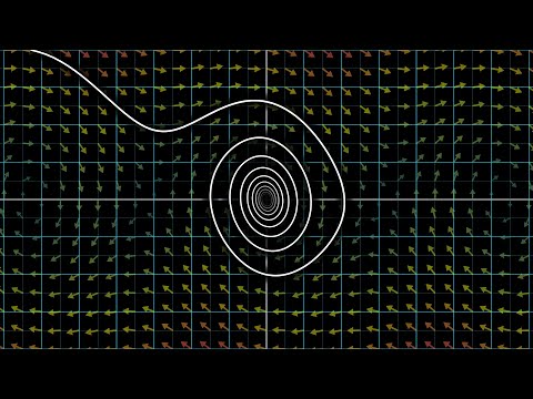
If you know the initial angle and the initial angular velocity, that's enough to predict how the system will evolve as time moves forward. If you haven't worked with them before, these sorts of diagrams can take a little getting used to. What you're looking at now, this inward spiral, is a fairly typical trajectory for our pendulum. So take a moment to think carefully about what is being represented. Notice how at the start, as θ decreases, θ' gets more negative, which makes sense, because the pendulum moves faster in the leftward direction as it approaches the bottom.
Keep in mind, even though the velocity vector on this pendulum is pointed to the left, the value of that velocity is always being represented by the vertical component of our space. It's important to remind yourself that this state space is an abstract thing, and it's distinct from the physical space where the pendulum itself lives and moves. Since we're modeling this as losing some of its energy to air resistance, this trajectory spirals inward, meaning the peak velocity and peak displacement each go down a bit with each swing. Our point is, in a sense, attracted to the origin, where θ and θ-dot both equal 0. With a space, we can visualize a differential equation as a vector field. Here, let me show you what I mean.
The pendulum state is a vector, theta, theta-dot. Maybe you think of that as an arrow from the origin, or maybe you think of it as a point. What matters is that it has two coordinates, each a function of time. Taking the derivative of that vector gives you its rate of change, the direction and speed that it will tend to move in this diagram. That derivative is a new vector, θ'θ'', which we visualize as being attached to the relevant point in space. Take a moment to interpret what this is saying. The first component for this rate of change vector is θ', which is also a coordinate in our space.
So the higher up we are in the diagram, the more the point tends to move to the right, and the lower we are, the more it tends to move to the left. The vertical component is theta-double-dot, which our differential equation lets us rewrite entirely in terms of theta and theta-dot itself. In other words, the first derivative of our state vector is some function of that vector itself, with most of the intricacy tied up in that second coordinate. Doing the same at all points of this space will show how that state tends to change from any position. artificially scale down the vectors when we draw them to prevent clutter, but use color to loosely indicate magnitude.
Notice, we've effectively broken up a single second-order equation into a system of two first-order equations. You might even give theta-dot a different name, to emphasize that we're really thinking of two separate values, intertwined via this mutual effect they have on one another's rate of change. This is a common trick in the study of differential equations. Instead of thinking about higher order changes of a single value, we often prefer to think of the first derivative of vector values. In this form, we have a wonderful visual way to think about what solving the equation means.
As our system evolves from some initial state, our point in the space will move along some trajectory in such a way that at every moment, the velocity of that point matches the vector from this field. And again, keep in mind, this velocity is not the same thing as the physical velocity of the pendulum, it's a more abstract rate of change, encoding the rates of change for both theta and theta-dot. You might find it fun to pause for a moment and think through what exactly some of these trajectory lines say about the possible ways the pendulum evolves from different starting conditions.
For example, in regions where θ-dot is quite high, the vectors guide the point to travel to the right quite a ways before settling down into an inward spiral. This corresponds to a pendulum with a high enough initial velocity that it fully rotates around several times before settling into a decaying back and forth. Having a little more fun? When I tweak this air resistance term, mu, say increasing it, you can immediately see how this will result in trajectories that spiral inward faster, which is to say the pendulum slows down faster. That's obvious when I call it the air resistance term, but imagine that you saw these equations out of context, not knowing that they described a pendulum.
It's not obvious just looking at them that increasing this value of mu will result in a trajectory that spins outward faster. It's not obvious just looking at them that increasing this value of mu will result in means that the system as a whole tends towards some attracting state faster. So getting some software to draw these vector fields for you can be a great way to build an intuition for how they behave. What's wonderful is that any system of ordinary differential equations can be described by a vector field like this, so it's a very general way to get a feel for them. Usually though, they have many more dimensions. For example, consider the famous three-body problem.
which is to predict how three masses in three-dimensional space evolve if they act on each other with gravity, and if you know their initial positions and velocities. Each mass has three coordinates describing its position, and three more describing its momentum. So the system has 18 degrees of freedom in total, and hence an 18-dimensional space of possible states. It's a bizarre thought, isn't it? A single point meandering through an 18-dimensional space that we cannot visualize, obediently taking steps through time based on whatever vector it happens to be sitting on from moment to moment, completely encoding the positions and momenta of the three masses we see in ordinary, physical 3D space.
In practice, by the way, you can reduce the number of dimensions here by taking advantage of the symmetries of your setup, but the point that more degrees of freedom result in higher dimensional state spaces remains the same. In math, we often call a space like this a phase space. You'll hear me use that term broadly for spaces encoding all kinds of states of changing systems, but you should know that in the context of physics, especially Hamiltonian mechanics, the term is often reserved for a more special case, namely a space whose axes represent position and momentum. so a physicist would agree that the 18-dimensional space describing the three-body problem is a phase space.
But they might ask that we make a couple of modifications to our pendulum setup for it to properly deserve the term. For those of you who just watched the block collision video, the planes we worked with there would happily be called phase spaces by math folk, though a physicist might prefer other terminology. Just know that the specific meaning may depend on your context. It may seem like a simple idea, depending on how well indoctrinated you are to modern ways of thinking about math, but it's worth keeping in mind that it took humanity quite a while to really embrace thinking of dynamics spatially like this, especially when the dimensions get very large.
In his book Chaos, the author James Glick describes phase space as one of the most powerful inventions of modern science. One reason it's powerful is that you can ask questions not just about a single initial condition, but about a whole spectrum of initial states. The collection of all possible trajectories is reminiscent of a moving fluid, so we call it phase flow. To take one example of why phase flow is a fruitful idea, idea, consider the question of stability. The origin of our space corresponds to the pendulum standing still, and so does this point over here, representing when the pendulum is perfectly balanced upright.
These are the so-called fixed points of our system, and one natural question to ask is whether or not they're stable. That is, will tiny nudges to the system result in a state that tends back towards that fixed point, or away from it? Physical intuition for the pendulum makes the answer here kind of obvious, but how would you think about stability just looking at the equations, say if they arose in some completely different less intuitive context? We'll go over how to compute the answers to questions like this in following videos, and the intuition for the relevant computations are guided heavily by the thought of looking at small regions in space around a fixed point, and asking whether the flow tends to contract or expand.
And speaking of attraction and stability, let's take a brief sidestep to talk about love. The Strogatz quote I mentioned earlier comes from a whimsical column in the New York Times on the mathematics of modeling affection, an example well worth pilfering to illustrate that we're not just talking about physics here.
Imagine you've been flirting with someone, but there's been some frustrating inconsistency to how mutual your affection seems, and perhaps during a moment when you turn your attention towards physics to keep your mind off the romantic turmoil, mulling over the broken up pendulum equations, you suddenly understand the on-again off-again dynamics of your flirtation, You've noticed that your own affection tends to increase when your companion seems interested in you, but decrease when they seem colder. That is, the rate of change for your love is proportional to their feelings for you. But this sweetheart of yours is precisely the opposite, strangely attracted to you when you seem uninterested, but turned off once you seem too keen.
The phase space for these equations looks very similar to the center part of your pendulum diagram. The two of you will go back and forth between affection and repulsion in an endless cycle. A metaphor of pendulum swings in your feelings would not just be apt, but mathematically verified. In fact, if your partner's feelings were further slowed when they feel themselves too in love, let's say out of a fear of being made vulnerable, we'd have a term matching the friction in the pendulum. and U2 would be destined to an inward spiral towards mutual ambivalence. I hear wedding bells already.
The point is that two very different seeming laws of dynamics, one from physics involving a single variable, and another from, uh, chemistry, with two variables, actually have a very similar structure, easier to recognize when you're looking at the phase diagram. Most notably, even though the equations are different, for example there's no sine function in the Romance equations, the phase space exposes an underlying similarity nevertheless. In other words, you're not just studying a pendulum right now, the tactics you develop to study one case have a tendency to transfer to many others.
OK, so phase diagrams are a nice way to build understanding, but what about actually computing the answer to our equation? Well, one way to do this is to essentially simulate what the universe would do, but using finite time steps instead of the infinitesimals and limits defining calculus. The basic idea is that if you're at some point in this phase diagram, take a step based on the vector you're sitting on for a small time step, delta t. Specifically, take a step equal to delta t times that vector. As a reminder, in drawing these vector fields, the magnitude for each vector has been artificially scaled down to prevent clutter.
But when you do this repeatedly, your final location will be an approximation of θt, where t is the sum of all those time steps. If you think about what's being shown right now, though, and what that would imply for the pendulum's movement, you'd probably agree that this is grossly inaccurate. But that's only because the time step delta-t of 0. 5 is way too big. If we turned it down, say to 0. 01, you can get a much more accurate approximation, it just takes more repeated steps is all. In this case, computing theta of 10 requires 1000 little steps.
Luckily we live in a world with computers, so repeating a simple task a thousand times is as simple as articulating that task with a programming language. In fact, let's finish things off by writing a little Python program that computes theta of t for us. What it has to do is make use of the differential equation, which returns the second derivative of theta as a function of theta and theta-dot. You start off by defining two variables, θ and θ dot, each in terms of some initial conditions. In this case, I'll have θ start at π thirds, which is 60 degrees, and θ dot start at 0. Next, write a loop that corresponds to taking many variables.
little time steps between 0 and your time t, each of size delta-t, which I'm setting here to be 0. 01. In each step of this loop, increase theta by theta-dot times delta-t, and increase theta-dot by theta-double-dot times delta-t, where theta-double-dot can be computed based on the differential equation. After all these little time steps, simply return the value of theta. This is called solving a differential equation numerically. Numerical methods can get way more sophisticated and intricate than this to better balance the tradeoff between accuracy and efficiency, but this loop gives the basic idea. So even though it sucks that we can't always find exact solutions, there are still meaningful ways to study differential equations in the face of this inability.
In the following videos, we will look at several methods for finding exact solutions when it's possible, but one theme I'd like to focus on is how these exact solutions can also help us study the more general unsolvable cases. But it gets worse. Just as there's a limit to how far exact analytic solutions can get us, one of the great fields to have emerged in the last century, chaos theory, has exposed that there are further limits on how well we can use these systems for prediction with or without solutions. Specifically, we know that for some systems, small variations to the initial conditions, say the kind due to necessarily imperfect measurements, result in wildly different trajectories.
We've even built some good understanding for why this happens. The three-body problem, for example, is known to have seeds of chaos within it. So looking back at the quote from earlier, it seems almost cruel of the universe to fill its language with riddles that we either can't solve, or where we know any solution would be useless for long-term prediction anyway. It is cruel, but then again it should also be reassuring. It gives some hope that the complexity we see in the world around us can be studied somewhere in this math, and that it's not hidden away in the mismatch between model and reality. .
S K R Y B O T
Skrybot. 2023, Transkrypcje video z YouTube
Informujemy, że odwiedzając lub korzystając z naszego serwisu, wyrażasz zgodę aby nasz serwis lub serwisy naszych partnerów używały plików cookies do przechowywania informacji w celu dostarczenie lepszych, szybszych i bezpieczniejszych usług oraz w celach marketingowych.